Time Series Machine Learning

Time series data is a crucial component of many real-world applications, from finance to healthcare. While its sequential nature adds complexity, transforming time series into a tabular format enables the application of traditional machine learning (ML) techniques.

In this blog, we’ll explore how to preprocess time series data and extract meaningful features, paving the way for powerful predictive pipelines.

Understanding Time Series Data

In data analytics, structured data often appears in a tabular format, where rows represent observations and columns represent attributes of those observations. For example, a patient dataset might have rows for individual patients and columns for properties such as age, diagnosis, and medication history. This structure facilitates efficient querying and analysis.

Time series data is also structured but differs due to its inherent temporal ordering. While conventional tabular data captures static attributes at a specific point, time series data tracks the evolution of an attribute over time. As such, one can conceptually represent time series in a 3D tabular format:

• Rows: Observations (e.g., recordings)
• Columns: Attributes (e.g., sensors)
• Third Dimension: Temporal measurements for each attribute

Note: While this 3D format is useful conceptually, time series data is rarely structured this way in practice.

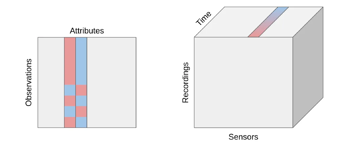Figure 1: Comparison of conventional tabular data (left) and conceptual time series structure (right).

Preprocessing and Feature Extraction

Preparing time series data for machine learning typically involves two steps: preprocessing and feature extraction.

Preprocessing

Preprocessing focuses on cleaning or transforming the raw time series data, including filtering noise, detrending, clipping outliers, and resampling. In practice, this step involves sequentially applying functions, which take time series data as input and output processed time series data, with the aim of preparing the data for further analysis or modelling in machine learning.

Feature Extraction

Feature extraction is concerned with extracting a set of meaninful characteristics (i.e., features) from the data, such as mean or spectral entropy. These features are calculated by applying functions (often in parallel). Unlike processing, feature extraction results in a tabular output that facilitates machine learning by creating a lower-dimensional representation of the time series data. In other words, the extracted features can be compiled into a feature matrix, which a 2D table where:

• Rows: observations or segments (windows) of the time series
• Columns: feature values derived from each segment

Multi-Domain Features

Features extracted on time series data can be derived from multiple domains;

• Temporal (statistical) measures: Mean, standard deviation, skewness
• Spectral features: Spectral entropy, frequency components

By combining features from various domains, one can create a very expressive representation of the time series.

Window-Based Feature Extraction

Given the relative simplicity of processing itself, i.e., transforming time series data into (processed) time series data, we will now focus on feature extraction.

One popular approach for feature extraction is the window-based approach, where a time series is segmented into smaller parts, or windows, which may overlap. Features are computed for each of these windows.

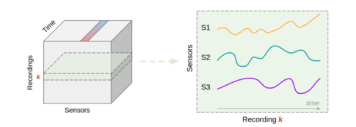Figure 2: Conceptual representation of time series signals (e.g., S1, S2, and S3) for a single recording.

Two primary types of window-based feature extraction are:

1. Full Window Feature Extraction
   The entire time series is treated as a single window, and features are extracted for the entire sequence. For each recording (which is a single window), a single row is added to the feature matrix containing the extracted features across all sensors.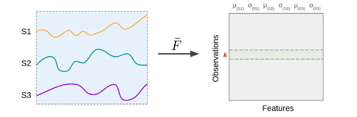

   Figure 3: Full window feature extraction. For each sensor, two features (μ and σ) are extracted over the entire time series.

2. Sliding Window Feature Extraction
   The time series is divided into overlapping or non-overlapping windows, and features are extracted for each segment. Two parameters govern this process:

   • Window size: The duration or length of each segment
   • Stride: The overlap or gap between successive windows For each window, a row is added to the feature matrix containing the extracted features across all sensors.

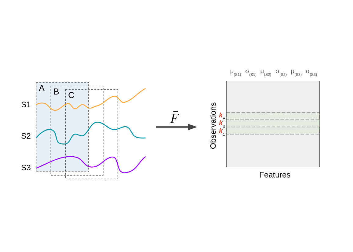
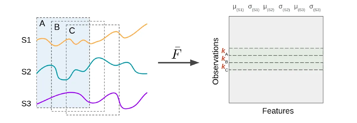   Figure 4: Sliding window feature extraction. For each sensor, two features (μ and σ) are extracted over each window.

More genarlized, we observe that for each window (segment) of the time series, a row is added to the feature matrix containing the extracted features across all sensors. The resulting feature matrix aligns with a traditional tabular format (rows=windows, columns=feature values), enabling the application of classical ML algorithms.

Multi-Resolution Feature Extraction

An interesting extension of window-based feature extraction is multi-resolution feature extraction, where features are extracted using different window sizes (i.e., at multiple resolutions). By varying the window size, the temporal context captured by the features is adjusted, allowing for the capture of both global trends and local patterns in the time series data.

Conclusion

Time series data’s sequential nature poses unique challenges, but transforming it into a tabular format enables the application of traditional machine learning. By preprocessing and extracting features, you can effectively represent time series data in a structured format suitable for traditional ML algorithms. Moreover, using multi-domain and multi-resolution features has been shown to be curcial in creating powerful predictive pipelines.

Let it not be a coincidence that tsflex (one of our open-source contributions) is a library that facilitates flexible and efficient extraction of multi-domain and multi-resolution features from time series data.